Clingraph package quick start with Jupyter#
We present in this notebook the basic functionalities of clingraph used as a package.
Try it yourself! Launch this notebook in Binder
We suggest that the user first gets familiarized with the accepted syntax.
The details on the package options are in api documentation.
For the command line usage see our command line documentation.
Our examples folder contains all the range of functionalities in different applications (Each subfolder contains a README that explains how to run it).
Python package functionality#
Load facts#
We use the Factbase class to gather all the facts defining the graphs
[1]:
from clingraph.orm import Factbase
Create a factbase from string#
Loads a string of facts
[2]:
fb = Factbase()
fb.add_fact_string('''
node(oscar).
node(andres).
edge((oscar,andres)).
attr(node,andres,label,"Andres").
attr(node,oscar,label,"Oscar").
attr(edge,(oscar,andres),label,"friends").''')
Show the facts after preprocessing
[3]:
print(fb)
node(oscar,default).
node(andres,default).
attr(edge,(oscar,andres),(label,-1),"friends").
attr(node,andres,(label,-1),"Andres").
attr(node,oscar,(label,-1),"Oscar").
edge((oscar,andres),default).
graph(default).
Create a Factbase from file#
The file contents representing two different graphs.
[4]:
!cat examples/doc/example2/example2.lp
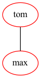
graph(toms_family).
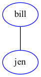
graph(bills_family).
node(tom, toms_family).
node(max, toms_family).
edge((tom, max), toms_family).
node(bill, bills_family).
node(jen, bills_family).
edge((bill, jen), bills_family).
Load the facts in the file#
[5]:
fb = Factbase()
fb.add_fact_file("examples/doc/example2/example2.lp")
Add additional facts#
[6]:
fb.add_fact_string("attr(graph_nodes,toms_family,color,red).attr(graph_nodes,bills_family,color,blue).")
Show all the facts
[7]:
print(fb)
edge((tom,max),toms_family).
edge((bill,jen),bills_family).
graph(toms_family).
graph(bills_family).
node(tom,toms_family).
node(max,toms_family).
node(bill,bills_family).
node(jen,bills_family).
attr(graph_nodes,bills_family,(color,-1),blue).
attr(graph_nodes,toms_family,(color,-1),red).
Graphviz functionality#
Compute the graphs#
[8]:
from clingraph.graphviz import compute_graphs
Computes the graphviz objects by calling compute_graphs(fb).
[9]:
graphs = compute_graphs(fb)
Show the cligraph objects
[10]:
print(graphs)
{'toms_family': <graphviz.graphs.Graph object at 0x7fb91df31220>, 'bills_family': <graphviz.graphs.Graph object at 0x7fb91df77c70>}
[11]:
graphs['toms_family']
[11]:

[12]:
graphs['bills_family']
[12]:

Get the source code#
This source code uses the DOT Language
[13]:
from clingraph.graphviz import dot
[14]:
dot_graphs = dot(graphs)
dot_graphs
[14]:
{'toms_family': 'graph toms_family {\n\tnode [color=red]\n\ttom\n\tmax\n\ttom -- max\n}\n',
 'bills_family': 'graph bills_family {\n\tnode [color=blue]\n\tbill\n\tjen\n\tbill -- jen\n}\n'}
[15]:
print(dot_graphs['toms_family'])
graph toms_family {
        node [color=red]
        tom
        max
        tom -- max
}
Write the dot in files#
Writes in one file per graph
[16]:
from clingraph.utils import write
[17]:
write(dot_graphs,directory="out",format="dot",name_format="source_{graph_name}")
File saved in out/source_toms_family.dot
File saved in out/source_bills_family.dot
Render the graphs#
We use IPython here only to display the output
[18]:
from IPython.display import Image
[19]:
from clingraph.graphviz import render
[20]:
render(graphs,format="png")
Image saved in out/toms_family.png
Image saved in out/bills_family.png
[21]:
Image("out/toms_family.png")
[21]:
[22]:
Image("out/bills_family.png")
[22]:
Create an animation in gif#
[24]:
from clingraph.gif import save_gif
[25]:
save_gif(graphs)
Image saved in out/images/gif_image_toms_family_0.png
Image saved in out/images/gif_image_bills_family_0.png
Gif saved in out/movie.gif
[26]:
Image("out/movie.gif")
[26]:
<IPython.core.display.Image object>
Generate latex code#
[27]:
from clingraph.tex import tex
[28]:
tex_graphs=tex(graphs)
tex_graphs
[28]:
{'toms_family': "\\documentclass{article}\n\\usepackage[x11names, svgnames, rgb]{xcolor}\n\\usepackage[utf8]{inputenc}\n\\usepackage{tikz}\n\\usetikzlibrary{snakes,arrows,shapes}\n\\usepackage{amsmath}\n%\n%\n\n%\n\n%\n\n\\begin{document}\n\\pagestyle{empty}\n%\n%\n%\n\n\\enlargethispage{100cm}\n% Start of code\n% \\begin{tikzpicture}[anchor=mid,>=latex',line join=bevel,]\n\\begin{tikzpicture}[>=latex',line join=bevel,]\n  \\pgfsetlinewidth{1bp}\n%%\n\\pgfsetcolor{black}\n  % Edge: tom -- max\n  \\draw [] (27.0bp,71.697bp) .. controls (27.0bp,60.846bp) and (27.0bp,46.917bp)  .. (27.0bp,36.104bp);\n  % Node: tom\n\\begin{scope}\n  \\definecolor{strokecol}{rgb}{1.0,0.0,0.0};\n  \\pgfsetstrokecolor{strokecol}\n  \\draw (27.0bp,90.0bp) ellipse (27.0bp and 18.0bp);\n  \\definecolor{strokecol}{rgb}{0.0,0.0,0.0};\n  \\pgfsetstrokecolor{strokecol}\n  \\draw (27.0bp,90.0bp) node {tom};\n\\end{scope}\n  % Node: max\n\\begin{scope}\n  \\definecolor{strokecol}{rgb}{1.0,0.0,0.0};\n  \\pgfsetstrokecolor{strokecol}\n  \\draw (27.0bp,18.0bp) ellipse (27.0bp and 18.0bp);\n  \\definecolor{strokecol}{rgb}{0.0,0.0,0.0};\n  \\pgfsetstrokecolor{strokecol}\n  \\draw (27.0bp,18.0bp) node {max};\n\\end{scope}\n%\n\\end{tikzpicture}\n% End of code\n\n%\n\\end{document}\n%\n\n\n",
 'bills_family': "\\documentclass{article}\n\\usepackage[x11names, svgnames, rgb]{xcolor}\n\\usepackage[utf8]{inputenc}\n\\usepackage{tikz}\n\\usetikzlibrary{snakes,arrows,shapes}\n\\usepackage{amsmath}\n%\n%\n\n%\n\n%\n\n\\begin{document}\n\\pagestyle{empty}\n%\n%\n%\n\n\\enlargethispage{100cm}\n% Start of code\n% \\begin{tikzpicture}[anchor=mid,>=latex',line join=bevel,]\n\\begin{tikzpicture}[>=latex',line join=bevel,]\n  \\pgfsetlinewidth{1bp}\n%%\n\\pgfsetcolor{black}\n  % Edge: bill -- jen\n  \\draw [] (27.0bp,71.697bp) .. controls (27.0bp,60.846bp) and (27.0bp,46.917bp)  .. (27.0bp,36.104bp);\n  % Node: bill\n\\begin{scope}\n  \\definecolor{strokecol}{rgb}{0.0,0.0,1.0};\n  \\pgfsetstrokecolor{strokecol}\n  \\draw (27.0bp,90.0bp) ellipse (27.0bp and 18.0bp);\n  \\definecolor{strokecol}{rgb}{0.0,0.0,0.0};\n  \\pgfsetstrokecolor{strokecol}\n  \\draw (27.0bp,90.0bp) node {bill};\n\\end{scope}\n  % Node: jen\n\\begin{scope}\n  \\definecolor{strokecol}{rgb}{0.0,0.0,1.0};\n  \\pgfsetstrokecolor{strokecol}\n  \\draw (27.0bp,18.0bp) ellipse (27.0bp and 18.0bp);\n  \\definecolor{strokecol}{rgb}{0.0,0.0,0.0};\n  \\pgfsetstrokecolor{strokecol}\n  \\draw (27.0bp,18.0bp) node {jen};\n\\end{scope}\n%\n\\end{tikzpicture}\n% End of code\n\n%\n\\end{document}\n%\n\n\n"}
Create a clingraph from each model retuned in the clingos solve#
This is achived my passing a function that gathers all Factbases in a list to the on_model callback argument for solve.
In this case our program has two stable models. One with node(a) and the other one with node(b)
[29]:
from clingo import Control
ctl = Control(["-n2"])
fbs = []
ctl = Control(["-n2"])
ctl.add("base", [], "1{node(a);node(b)}1.")
ctl.ground([("base", [])])
ctl.solve(on_model=lambda m: fbs.append(Factbase.from_model(m)))
[29]:
SolveResult(1)
Now we have a list of Factbase objects that can be passed to any of the above functions
[30]:
print(fbs)
[<clingraph.orm.Factbase object at 0x7fb91e64c1f0>, <clingraph.orm.Factbase object at 0x7fb91e64cee0>]
[31]:
graphs = compute_graphs(fbs)
graphs
[31]:
[{'default': <graphviz.graphs.Graph at 0x7fb91e4387f0>},
 {'default': <graphviz.graphs.Graph at 0x7fb91e8b9940>}]
[32]:
render(graphs,name_format="{model_number}/multi-{graph_name}",format='png')
Image saved in out/0/multi-default.png
Image saved in out/1/multi-default.png
[33]:
Image('out/0/multi-default.png')
[33]:

[34]:
Image('out/1/multi-default.png')
[34]:
