Command line functionality#
Clingraph provides command line functionality to generate graphs from files and standard input. The graphs can then be printed as a dot string, rendered, converted into a gif or into latex code.
Special integration for clingo includes the creation of graphs from multiple stable models using clingos’ json output format.
Note
For advanced examples on how to use the command line see our examples folder. Each subfolder contains a README explaining how to run the example.
The command line usage is described below. However, the latest available options can be found by running:
$ clingraph --help
Loading facts#
The input can be loaded from multiple files and standard input, following our syntax. Any additional predicates will be ignored. Additionally, a single JSON file can be provided instead, with the structure of clingos json output format with –outf=2. More details can be found in clingo integration
Example
Consider the example1.lp
node(john).
node(jane).
edge((john,jane)).

node(joe).
edge((john,joe,1)).
edge((john,joe,2)).

attr(graph, default, label, "Does family").

attr(graph_nodes, default, style, filled).
attr(node, john, label, "John Doe").
attr(node, jane, label, "Jane Doe").
Load from a file
$ clingraph example1.lp
Load from from stdin
$ cat example1.lp | clingraph
node(john,default).
node(jane,default).
attr(node,jane,(label,-1),"Jane Doe").
attr(node,john,(label,-1),"John Doe").
attr(graph,default,(label,-1),"Does family").
attr(graph_nodes,default,(style,-1),filled).
edge((john,jane),default).
graph(default).
Output#
Output formats#
- Clingraph provides four types of outputs
facts: Shows all the facts provided that are part of the syntax, after preprocessingdot: Generates the graphviz objects and prints the source DOT languagerender: Generates the graphviz objects and renders the imagestex: Generates the graphviz objects and prints the latex codeanimate: Generates the graphviz objects and creates an animation in gif format
Example
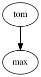
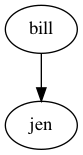
Consider the example2.lp
    graph(toms_family).
    graph(bills_family).

    node(tom, toms_family).
    node(max, toms_family).
    edge((tom, max), toms_family).

    node(bill, bills_family).
    node(jen, bills_family).
    edge((bill, jen), bills_family).
Facts output
out=facts
The output is a string containing the facts for all graphs provided that are part of the syntax, after preprocessing
Example
$ clingraph example2.lp --out=facts
node(tom,toms_family).
node(max,toms_family).
node(bill,bills_family).
node(jen,bills_family).
graph(toms_family).
graph(bills_family).
edge((tom,max),toms_family).
edge((bill,jen),bills_family).
Dot output
out=dot
The output is a string containing the graph in DOT language
Example
$ clingraph example2.lp --out=dot
graph toms_family {
  tom
  max
  tom -- max
}

graph bills_family {
  bill
  jen
  bill -- jen
}
Output can also be saved in an individual files per graph with argument --save.
The file is saved in directory --dir and using the name formatting --name-format.
Example
$ clingraph example2.lp --out=dot --save --dir='out' --name-format='new_version_{graph_name}'
File saved in out/new_version_toms_family.dot
File saved in out/new_version_bills_family.dot
Render output
out=render
The graphs will be rendered and saved in files with a given format and engine
Example
$ clingraph example2.lp --out=render --format=png
Image saved in out/toms_family.png
Image saved in out/bills_family.png
Animate output
out=animate
- Generates an animation with the graph rendering. The order of the images can be provided with argument
--sortbased on the name. asc-str: Sort ascendent based on the graph name as a stringasc-int: Sort ascendent based on the graph name as an integerdesc-str: Sort descendent based on the graph name as a stringdesc-int: Sort descendent based on the graph name as an integername1,...,namex: A string with the order of the graph names separated by ,
Additionally the number of frames per second can be set with --fps.
Example
$ clingraph example2.lp --out=animate --sort=desc --name-format=families_gif
Image saved in out/images/gif_image_toms_family_0.png
Image saved in out/images/gif_image_bills_family_0.png
Gif saved in out/families_gif.gif
Latex output
out=tex
See the latex integration section.
Partial output#
Graphs can be selected by name to work only with a subset of the output using argument –selected-graphs
Example
$ clingraph example2.lp --out=dot --select-graph=toms_family
graph toms_family {
  tom
  max
  tom -- max
}
Clingo integration#
These features allow the usage of logic programs with rules to define the visualization. This is done in integration with clingo, letting the user handle multiple stable models.
Tip
Good practices
We advice the user to keep the visualization encoding separate from the encodings used to solve the problem. This visualization encoding can include rules but no choices, those should be handled in the encoding.
Example
Consider the encoding example5_encoding.lp that has two stable models.
1{person(a);person(b)}1.
And a different file example5_viz.lp for the visualization encoding.
node(X):-person(X).
attr(node,a,color,blue):-node(a).
attr(node,b,color,red):-node(b).
Piping json output#
Warning
This integration only supports special characters in strings, such as escaped quotes attr(node,a,label,"Quotes\""), when using clingo >= 5.5.2.
Run clingo to obtain the two stable models formatted as json with option
--outf=2
Example
$ clingo example5_encoding.lp example5_viz.lp -n0 --outf=2
{
  "Solver": "clingo version 5.5.2",
  "Input": [
    "examples/doc/example5/example5_encoding.lp","examples/doc/example5/example5_viz.lp"
  ],
  "Call": [
    {
      "Witnesses": [
        {
          "Value": [
            "node(a)", "person(a)", "attr(node,a,color,blue)"
          ]
        },
        {
          "Value": [
            "node(b)", "person(b)", "attr(node,b,color,red)"
          ]
        }
      ]
    }
  ],
  "Result": "SATISFIABLE",
  "Models": {
    "Number": 2,
    "More": "no"
  },
  "Calls": 1,
  "Time": {
    "Total": 0.001,
    "Solve": 0.000,
    "Model": 0.000,
    "Unsat": 0.000,
    "CPU": 0.001
  }
}
Pipe clingo’s json output to clingraph
Example
$ clingo example5_encoding.lp example5_viz.lp -n0 --outf=2 | clingraph --out=dot
WARNING:  - Outputing multiple models in stdout.
graph default {
  a [color=blue]
}

graph default {
  b [color=red]
}
Load a json file
Example
$ clingo example5_encoding.lp example5_viz.lp -n0 --outf=2 > out/example5.json ; clingraph out/example5.json --out=dot
WARNING:  - Outputing multiple models in stdout.
graph default {
  a [color=blue]
}

graph default {
  b [color=red]
}
Select a single model using the model number starting with index 0
Example
$ clingo example5_encoding.lp example5_viz.lp -n0 --outf=2 | clingraph --out=dot --select-model=1
graph default {
  b [color=red]
}
Define the visualization encoding#
The visualization encoding can also be provided as a separate argument --viz-encoding.
This allows for integration projects using more complex scripts or applications.
When passing a json as input, the visualization facts will be obtained by running clingo with the visualization encoding for each stable model.
Furthermore, the functions defined in ClingraphContext will be available for usage withing the encoding preceded by @.
Warning
The visualization encoding should not include any choices, only the first stable model will be considered.


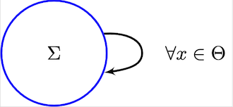
Latex integration#
The integration generates latex code for the graphs using the dot2tex package. This feature allows the user to include mathematical notation in the labels.
Warning
To use math notation ($) in labels, we advise the user to use the texlbl special attribute for the latex label instead of the normal label attribute. This will avoid problems with the escape characters. Note that edges require a label attribute to be defined (even if it is empty) in order for the texlbl attribute to have an effect. Additionally, the backslash \ must be escaped.
Example
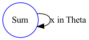
Consider the example6.lp
node(sum).
attr(node,sum,label,"Sum").
attr(node,sum,texlbl,"$\\Sigma $").
attr(node,sum,shape,circle).
attr(node,sum,color,blue).
edge((sum,sum)).
attr(edge,(sum,sum),texlbl,"$\\forall x\\in \\Theta$").
attr(edge,(sum,sum),label,"x in Theta").
Run cligraph to obtain the latex file using the output option --out=tex.
The optional parameters in --tex-param are passed to dot2tex.
This parameter should be a string arg_name=arg_value.
Then, the compilation can be done using a package like pdflatex